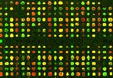
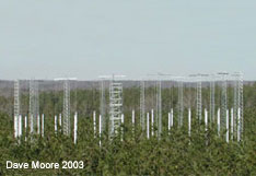
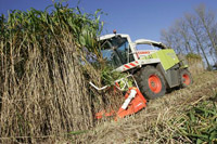
Some notes on statistical analysis at FACTS-1 regarding RBAI (relative basal area increment), biomass increment, NPP and litterfall

David J. Moore, BSc.
Program in Ecology and Evolutionary Biology
University of Illinois at Urbana-Champaign

Moore et al. "Inter-annual variation in the response of tree growth and productivity of a Pinus taeda forest exposed to elevated CO2" submitted to Global Change Biology in 2004.

Abstract

Rising CO2 is predicted to increase forest productivity, though the duration of the response and how it might change with fluctuations in rainfall and temperature is not clear.  We used repeated measures of diameter growth and allometric scaling to estimate the effect of Free Air Carbon-dioxide Enrichment (FACE) on tree growth and net primary production (NPP) in a rapidly growing Pinus taeda plantation over 6 years. Elevated CO2 increased the relative basal area increment (RBAI) of individual trees and NPP by between 5.7 % and 19.5 %. The growth stimulation was observed only in trees in the two intermediate size classes. Neither the smallest, suppressed trees nor the largest, emergent trees responded to elevated CO2 by increasing RBAI.  NPP in both ambient and elevated plots was positively correlated with rainfall during the growing season.  Unlike the relationship to precipitation, NPP was greatest in years of intermediate temperature, and the relative increases in RBAI and NPP in elevated CO2 were positively correlated with growing season degree day totals. An increase in the proportional response to elevated CO2 with increasing temperature is consistent with the predicted photosynthetic response of C3 plants. Exposure to elevated CO2 caused an average increase of NPP by 182 ± 28 g DM m^-2 y^-1 and biomass increment was increased by 100 ± 29 g DM m^-2 y^-1.  Because the growth rates of the largest trees in the forest did not respond to elevated CO2, its effect on productivity may diminish in future. Consequently, it is unlikely that increases in forest productivity globally will adequately offset increasing anthropogenic emissions of CO2.

The purpose of this document

The FACTS-1 experiment has provided one of the richest data-sets regarding the responses of forests to elevated CO2. One of the main goals of this experiment is to determine if forests will take up more carbon from the atmosphere as CO2 continues to rise. There are multiple sources of variation in forest ecosystems for example heterogeneous soil type and soil moisture, variation in tree density, differences in aspect and elevation. Because many of these factors can alter the growth rates of trees it is very important to explain as much variation as possible before we interpret the effects of elevated CO2.

A common way to account for inherent variation within a field site is to divide experimental plots into blocks which are areas of the field site which are as closely matched as possible. The blocking scheme at FACTS-1 has not been completely satisfactory and in our analysis we have found reliance on statistical blocking to be inadequate.

In this document I explain how we dealt with plot to plot differences at FACTS-1 and to underscore the need to account for these differences. The results from this analysis may be found in Moore et al. "Inter-annual variation in the response of tree growth and productivity of a Pinus taeda forest exposed to elevated CO2" submitted to Global Change Biology in 2004. Also I have included a draft of the materials and methods from that publication at the end of this document.

To determine if elevated CO2 increases net primary production in Pinus taeda we need to estimate the amount of biomass the pines produce in each year.

To calculate Biomass increment we need to do one of two things:

1. measure all the trees each year and scale dbh to biomass using allometric equations
2. measure a sub-sample of the trees each year, apply a growth rate calculated from this sub-sample to a one time measure of the dbh of all trees in the experiment, then scale from dbh to biomass using allometric equations.

We opt for number 2 because we have a long term record of the growth of about 30% of the trees in the experiment. This is a large sample size and a wide range of tree sizes were selected at the start of the experiment.

To get good estimates of NPP we need accurate and precise measurement of the trees  and accurate estimates of the growth rates this requires some thought.

As some have pointed out there is considerable variation between the plots in terms of growth rate, productivity and N content. This was highlighted by Schäfer et al. 2003 (Fig. 1 reproduced from Schäfer et al. 2003).

Going beyond blocking

Early estimates of the treatment effect in this forest may have been too high because the relative basal area increment declines as the number and size of neighboring trees increases (Fig.2). 

So we must account for this variation in any analysis carried out.

Our statistical model
 

To analyze the RBAI data for the effect of elevated CO₂ while accounting for the initial difference between plots we use the following model

RBAI =

year

initialBAtotal

initialBAtotal*year

sizeclass

sizeclass*year

treatment

year*treatment

sizeclass*treatment

year*treatment*sizeclass

And we include the following random factors

block block*treatment block*sizeclass block*sizeclass*treatment

This configuration essentially tells the model that N=3 blocks, and that trees within each block are split or grouped into four size classes.

(We can change these random factors a little i.e. we don’t need to include the sizeclass interaction with block in the model but it accounts for some variation so I left it in.  It changes the p values slightly but doesn’t change the outcome)

The most important thing here is that we are using the covariate to remove some of the variation we can’t account for by blocking.  Taking the covariate into account dampens the treatment effect.

Why did previous studies overestimate the treatment effect?

If you look at Fig. 2 and compare rings 1 and 2 you see that the treatment effect is small whereas if you compare rings 4 and 6 the treatment effect is large. However much of the difference between rings 4 and 6 can be attributed to variation in starting total basal area (the x axis).  This is why failure to account for this source of variation causes overestimation of the treatment effect.

Here’s an example….

This is the output from the model for RBAI of trees in each plot in 1998.

But much of the variation is caused by the initial basal area of the plot rather that the treatment so we take this into account by adding “total basal area” as a covariate.  First we test to see if the slope of the relationship between RBAI and total basal area differs

significantly between ambient and elevated CO2 and, having excluding this possibility, we assume that the slopes are the same.  Thus we have two parallel lines relating RBAI to

total basal area in both treatments (Fig. 4). The treatment effect is the vertical distance between these two lines or the difference in the ‘y’ intercept.

To estimate the basal area of the trees in each plot we use RBAI values to ‘grow’ the trees in each plot.  We measure the trees at one point in time (1998) and then apply the growth rates to each tree. We use allometric regression to convert dbh to biomass for each tree and sum the total biomass of each plot. 

Since RBAI is artificially inflated because of variation between the plots then using a different RBAI for each plot causes the biomass increments to be inflated in turn.

If we could remove the effect of CO2 stimulation how would the trees grow?  We can try to do this by going back to the previous example….

Next we will scale to stand level biomass increment using ONLY the lower ambient predictions for each plot (only the white dots in Fig.5). I will refer to this from now on as the NULL METHOD and we can compare the average of plots 1,5 & 6 with the average of 2,3 & 4 to see if there is a bias.

Previously RBAI values for each plot were used to calculate the biomass increment of each plot (DeLucia et al. 1999, Finzi et al. 2002, Hamilton et al. 2002). This did not account for the strong effect of starting total basal area on RBAI.  In Fig. 6 I compare the methods used in the published literature with the null method example from above…

 Reliance on averages (or any estimates that fail to account for the strong effect of total basal area on RBAI) causes an over estimate in the treatment effect.

How have we solved this problem?

Using RBAI estimates that are corrected for the covariate only goes part of the way – the size structure of the forest effects the RBAI biologically and the biomass estimates mathematically. 

The first thing we did was to use the covariate corrected RBAI values to ‘grow’ the trees in each plot.  This accounts for the error illustrated in Fig. 6 (lower curve) and results in a revised estimate which is lower than the initial over estimate (Fig. 7). 

We find even if we assume RBAI is the same for all plots, the size and distribution of the trees in plots 2, 3 & 4 results in more biomass production than in plots 1, 5 & 6 (lower line Fig. 8). 

To account for this we calculated how big the trees were in 1996 then we applied the ambient RBAI numbers (by size class) estimated for the treatment by the mixed model ANCOVA to every tree in all 6 rings. Then we repeated this using the elevated RBAI numbers.  This has the advantage of removing as much variation from the Biomass increment estimates as possible (Fig.8).

The ANCOVA results in an RBAI estimate for the ‘average’ level of the covariate which is the level for all six rings combined so the application of the RBAI from the ANCOVA is appropriate.

This new estimate is directly proportional to the mathematical difference between the initial over estimate and the null method bias (Fig. 9).

Materials and methods

Site description. This research was conducted at the FACTS-1 research site at Duke Forest in the Piedmont region of North Carolina (35^o58’N 79^o05’W). This facility uses FACE technology to increase the CO2 concentration in three of six experimental plots within a continuous unmanaged Pinus taeda plantation (Hendrey et al., 1999). Each plot is 30-m in diameter and consists of a circular plenum that delivers air to an array of 32 vertical pipes.  The pipes extend from the forest floor to above the 18-m tall forest canopy and contain adjustable ports at 50-cm intervals that allow control of atmospheric CO2 through the entire forest volume. 

CO2 enrichment occurred 80% of the time as it was switched off when air temperature was too cold for photosynthesis to occur (below 6^oC) and when windspeeds exceeded 5 m s^-1.  The average CO2 concentration (24h average) in the three fully instrumented control plots during the 6 years of the experiment was approximately 386 μmol mol^-1 and three experimental plots were maintained at ambient plus 196 μmol mol^-1 CO2 (approximately 582 μmol mol^-1 during active enrichment).  Seedlings were planted in 1983 in 2.4 m x 2.4 m spacing.  Since that time a number of hardwood species have established in the understory.  When fumigation began in August 1996, P. taeda trees were ~14 m tall and comprised more than 90% of the basal area of the stand.  This analysis was restricted to the P. taeda as this species accounts for over 85% of net primary production (NPP) in this forest (Hamilton et al., 2002).

Tree growth. In 1996 spring-loaded stainless steel dendrometer bands, for measuring diameter, were fitted to the boles of trees approximately 1.4 m above ground level (Keeland and Sharitz, 1993). Diameter was measured approximately monthly on between 31 and 34 trees in each plot (105 in the ambient plots and 104 in elevated plots). Bands were read in the same order each month and at the same time of day to reduce the effects of diurnal changes in diameter. The basal area increment (cm² month^-1) was calculated for each measurement period and normalized to a 30 day interval. The annual growth rate of each tree, expressed as relative basal area increment (RBAI,) was calculated as the change in basal area divided by the initial basal area for each year (Naidu and DeLucia, 1999). Because RBAI is a measure of relative growth (cm² cm^-2 yr^-1) units will be expressed as yr^-1. Trees with negative RBAI were assumed to be dead and were excluded from further analysis. There was no statistically significant difference in mortality in the control and treatment plots.

To account for potential differences in the response of different sized trees to CO2, individuals were grouped into 4 classes based on their basal area in 1996, with equal numbers of trees in each class. Trees in class I had a basal area smaller than 110 cm² and were competitively suppressed with most of their crowns below the canopy. Class II included trees between 110 cm² and 193 cm²; these trees were mostly co-dominant with their crowns defining the canopy. Class III (trees between 193 cm² and 270 cm²) and class IV (larger than 270 cm²) were a mixture of co-dominant and emergent individuals with crowns extending above the canopy.  Class III contained mostly co-dominant individuals with some emergent trees, while more than 75% of the trees in class IV were emergent.

Modeling initiation and termination of growth. To determine if the CO2 treatment and inter-annual variation in climate affected the timing and duration of diameter growth in P. taeda a mathematical model was used to estimate the start, end and duration of cambial expansion in each year. Two independent non-linear models (Proc Nlin, SAS v. 8.02, Cary, NC) for the start of growth and the end of growth, respectively, were fitted to the basal area measurements of each tree for each year of the experiment (Fig. 10).

For the period before the start of growth, basal area (BA) was defined as BA = a; and after the start of growth BA = a + b (days) + b² (days²), where a was the initial basal area, b was the slope of the linear portion of the increase in basal area and b² is the curvature of that increase.  The start day was defined mathematically as the intersection between these two functions (Fig. 10).

The end of growth was estimated in the same way except the end day was the intersection between the growth curve and the final basal area (Fig. 10). Because the stop model estimated the end of growth asymptotically we defined the end of the growing season as the day when BA was 90% of the annual maximum. 

Fig. 10. The change in basal area from December 1997 through April 1999 for a typical loblolly pine tree. Basal area was calculated from measurement of bole diameter (DBH). The symbols represent measured values and the lines represent models fit to the data. Two functions were used to describe the progression of growth from winter into summer and autumn (left panel). In winter, BA (basal area) = a (constant), and during summer and autumn, BA = a + b(day) + b²(day²); where b is the initial growth rate of the tree and b² is the curvature of growth late in the season. The intersection of these two functions defined the “start day”. The progression of growth from summer into the following winter was also described by two functions (right panel). During summer and autumn, BA = a1’ + b’(day) + b’²(day²) and during the following winter, BA = a’. The intersection of these two functions defined the ‘end day’.  The ‘end day’ was then modified to accommodate the gradual cessation of growth late in the year.

Net primary production. The only two components of net primary production (NPP) quantified every year were biomass increment (above- and below-ground biomass) and litterfall. Our estimate of NPP does not include fine root production, herbivory or the annual production of dissolved organic and volatile carbon (Clark et al., 2001). These components contribute less than 10% of NPP in this forest (Hamilton et al., 2002).

Biomass per unit ground area was estimated at the beginning and end of each year by applying site specific allometric regressions to the diameter of each tree (Naidu et al., 1998), and the biomass increment was the difference in these values. Different equations were used for dominant and suppressed trees (Naidu et al., 1998) and evidence to date indicates that the CO2 treatment has not affected the site-specific allometric regressions (DeLucia et al., 2002). The change in diameter of trees was calculated by applying the treatment least square mean RBAI for each size class to all trees in that size class in each plot. 

Litterfall was collected with 12 replicate 40 x 40 cm baskets in each plot as in Finzi et al., (2002); the basket contents were analyzed twice per month from September through December and once per month at other times. Litterfall was expressed on a ground-area basis by dividing the total mass of P. taeda litterfall for each plot by the area of ground covered by the baskets.  NPP was calculated by adding the mass of litterfall and the total biomass increment for each plot. Biomass increment, litterfall and NPP are expressed as total dry matter per unit ground area per year (g DM m^-2 y^-1)

Statistical analysis. Statistical analyses were conducted with the SAS System for Windows (SAS v. 8.02, Cary, NC). We used a repeated measures mixed model ANOVA (Proc Mixed) to estimate the fixed effects of CO2 treatment (2 levels: ambient and elevated), year (7 levels: 1996 to 2002) and size class (4 levels: I, II, III and IV) on the start, end and duration of the growing season, initial growth rate and annual RBAI. The block, block by treatment, block by size class and block by treatment by size class effects were considered random and the degrees of freedom were calculated using the Satterthwaite correction. The subject of the repeated measure was the individual tree and the covariance structure was modeled using an autoregressive heterogeneous variance–covariance matrix. 

The initial total basal area of each plot was included as a covariate in the model when analyzing RBAI because it strongly influenced RBAI and varied between experimental plots. Failure to account for this plot to plot variation caused treatment effects to be over estimated. 

Unless otherwise stated, all data presented are least square means estimated by restricted maximum likelihood analysis within a mixed model. Error bars are the standard error of the difference between least squared means of the treatment and control. Tests for the treatment effect in each year of the experiment were based on upper tailed linear contrasts.Tests for the treatment effect on different size classes were based on upper tailed linear contrasts.

Litterfall was analyzed similarly using a repeated measures mixed model ANOVA (Proc Mixed), but because litterfall is a stand level measurement the subject of the repeated measure was the individual plot and tree size classes were not included in the model. Both biomass increment and NPP were analysed using the same statistical model used for litterfall except that the covariate of initial total basal area was omitted as it had already been accounted for in the estimation of RBAI used to calculate biomass increment.

The relationships of annual biomass increment, litterfall, NPP, and the percent stimulation of RBAI and NPP, to temperature and rainfall were tested using regression analysis (Proc Reg). Analysis of covariance (ANCOVA, Proc Mixed) was used to determine if elevated CO2 affected the slopes of the regressions. If there was no interaction (p > 0.25) between the treatment and the environmental variable (rainfall or temperature) the interaction term was removed.

References

Clark DA, Brown S, Kicklighter DW, Chambers JQ, Thomlinson JR, Ni J (2001) Measuring net primary production in forests: Concepts and field methods. Ecological Applications, 11, 356-370.

DeLucia EH, Hamilton JG, Naidu SL et al. (1999) Net primary production of a forest ecosystem with experimental CO2 enrichment. Science, 284, 1177-1179.

DeLucia EH, George K, Hamilton JG (2002) Radiation-use efficiency of a forest exposed to elevated concentrations of atmospheric carbon dioxide. Tree Physiology 22, 1003-1010.

Finzi AC, DeLucia EH, Hamilton JG, Richter DD, Schlesinger WH (2002) The nitrogen budget of a pine forest under free air CO2 enrichment. Oecologia, 132, 567-578.

Hamilton JG, DeLucia EH, George K, Naidu SL, Finzi AC, Schlesinger WH (2002) Forest carbon balance under elevated CO2. Oecologia, 131, 250-260.

Hendrey GR, Kimball BA (1994) The Face Program. Agricultural and Forest Meteorology, 70, 3-14.

Hendrey GR, Ellsworth DS, Lewin KF, Nagy J (1999) A free-air enrichment system for exposing tall forest vegetation to elevated atmospheric CO2. Global Change Biology, 5, 293-309.

Keeland BD, Sharitz RR (1993) Accuracy of Tree Growth Measurements Using Dendrometer Bands. Canadian Journal of Forest Research-Revue Canadienne De Recherche Forestiere, 23, 2454-2457.

Naidu SL, DeLucia EH, Thomas RB (1998) Contrasting patterns of biomass allocation in dominant and suppressed loblolly pine. Canadian Journal of Forest Research-Revue Canadienne De Recherche Forestiere, 28, 1116-1124.

Naidu SL, DeLucia EH (1999) First-year growth response of trees in an intact forest exposed to elevated CO2. Global Change Biology, 5, 609-613.

Schäfer KVR, Oren R, Ellsworth DS, Lai CT, Herrick JD, Finzi AC, Richter DD, Katul GG (2003) Exposure to an enriched CO2 atmosphere alters carbon assimilation and allocation in a pine forest ecosystem. Global Change Biology, 9, 1378-1400.